MRF for image restoration

Actually we discussed how to use MRF for image restoration before. Here we'd like to talk more about how an image restoration problem can be formulated as MRF and how to solve it.

Given an observed (noisy and possibly corrupted) image $Y$, how to recover the original image $X$ is the image restoration problem. Here we set the image as binary, i.e. a pixel can only be either 0 or 1. MRF formulated it as an optimization problem:

$$\arg \min_XE(X, Y) = \arg \min_X ||Y - X|| - \beta\sum_{x_i, x_j \in N}(x_ix_j + (1 - x_i)(1 - x_j))$$

$x_i, x_j \in N$ means $x_i$ and $x_j$ are adjacent. That's also why Morkov appears in the model's name.

Energy function

There are several views to reach the final energy function.

A simple intuition is most natural images contain large smooth regions (or continuous regions in binary images). Therefore we use $-\sum_{x_i, x_j \in N}(x_ix_j + (1 - x_i)(1 - x_j))$ to penalize discontinuities in the image. Considering we are given an observation $Y$, a regularization factor $||Y-X||$ is used.

Besides regularization perspective, a generative model based on hidden variable can also achieve the same energy function. If we treat the "real" image without noise as a grid of hidden variables $X$, with each $x_i$ generating the observation $y_i$ with a Bernoulli distribution $p(y|x)$ (like the image below shows), the posterior of this model can be formulated as

$$p(X|Y) \propto p(Y|X)p(X) = \prod_i p(y|x=0)^{1 - x_i}p(y|x=1)^{x_i} \exp[\beta \sum_{x_i, x_j \in N}(x_ix_j + (1 - x_i)(1 - x_j))]$$

Note we also use $\exp[\sum_{x_i, x_j \in N}(x_ix_j + (1 - x_i)(1 - x_j))]$ as X's priori. Therefore,

$\ln p(X|Y) \propto \sum_i \lambda(y_i)x_i + \beta \sum_{x_i, x_j \in N}(x_ix_j + (1 - x_i)(1 - x_j))$

in which $\lambda(y_i) = \frac{\ln p(y_i|x_i=1)}{\ln p(y_i|x_i=0)}$. Note when $y_i=0$, $\lambda(y_i)<0$ thus $\lambda(y_i)x_i$ will be larger when $x_i=0$, and when $y_i=1$, $\lambda(y_i)>0$ thus $\lambda(y_i)x_i$ will be larger when $x_i=1$, the term $\lambda(y_i)x_i$ actually acts as a "correction cost", which corresponds to the regularization term in the first perspective. (We need to maximize $\ln p(X|Y)$ here. Please note the differences in signs.)

Another view is graphical model. MRF is a typical undirected graphical model, whose clique contains only two nodes (as the following figure shows). Thus it's easy to write out its potential function the same as $p(X|Y)$ above.

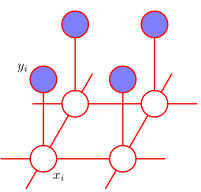
Graphical model view of Morkov Random Field, figure from Pattern Recognition and Machine Learning.

Solving MRF

A fairy simple approach to solve MRF is Iterated Conditional Modes (ICM), which optimizes each pixel in order with fixing all the other pixels. This approach can produce somehow good result, as last blog post shows (check the experiment part). But a problem is, it's easy to stuck in local minima. Fortunately, a clever transform of this optimization problem into finding a minimum cut in a graph, which appeared in 1989 and is called graph-cut, can produce a global optima.

As we saw in the energy function reduction, the image can be treated as a graph, in which vertices are pixels, and there are edges connecting neighbor pixels. If we add another two vertices, s (for the source) and t (for the sink) with some more edges, there will be a new graph which has interesting properties. The detailed rules to construct the new graph are:

• There are edges from s to every vertex whose observed pixel value is 0 (i.e. black pixels), with capacity as $\lambda(y_i = 0)$, and edges from every white pixels to t, with capacity $\lambda(y_i=1)$. These edges are called t-links.
• There are undirected edges between every two neighbor pixels, with capacity $\beta$, which are called n-links.

Therefore, if we divide all the vertices in the graph as two parts, one called S for it contains s, and the other called T for it contains t, there will be some edges connecting these two parts, which are called cut. This partition of the graph can be interpreted as, setting all the vertices along with s as black, and all the other pixels as white, i.e. $x_i = \begin{cases}0 & x_i \in S \\ 1 & x_i \in T \end{cases}$. Then this will become the final image $X$ after restoration. Let's check what's the overall capacity of the cut.

• For t-links, note only when $x_i \neq y_i$, can a t-link become a cut. Therefore $C_t(X) = \sum_{x_i \neq y_i}\lambda = \lambda||Y-X||$, which is the "correction cost" (or the likelihood) in the energy function.
• For n-links, if we set $w_{ij} = \beta(x_ix_j + (1-x_i)(1-x_j))$, $C_n(X) = \sum_{x_i \neq x_j} \beta = \sum_{x_i, x_j \in N} \beta(x_ix_j + (1-x_i)(1-x_j))$, which is the discontinuity penalty in the energy function.
• Therefore, $C(X) = C_t(X)+C_n(X)$ is exactly the energy function which we want to minimize.

Given the min-cut/max-flow theorem, it's easy to get the global optima in polynomial time, especially after Yuri et. al. proposes their fast algorithm.

I did some simple implementations. Here are the results. The first image is the noisy image, the second one is the result from ICM, and the third is from graph-cut. To my surprise, the C++-implemented graph-cut is even several times faster then MATLAB-implemented ICM.

Experiment result of MRF-based image restoration. The images are 1) input noisy image, 2) result from ICM, 3) result from graph-cut.

Insights?

How does graph-cut come up with this graph formulation? Are there any insights in it? In fact, what graph-cut does is:

• Use graph structure to indicate observations.
• Use some property of graphs to indicate energy functions.
• Take advantage of mature graph algorithm to optimize this property.

This seems extendable for other problems. Besides, MRF and HMM are very similar, MRF can be treated as a 2D extension of HMM from a hidden variable's perspective. The difference is, MRF views Morkov property in a spatial way, however, HMM interprets Morkov property as temporal order. What if we view MRF from a temporal perspective or extend it to 3D temporal-spatial MRF?